2. Simulators#

From the perspective of BayesFlow, a generative model is more than just a prior (encoding beliefs about the parameters before observing data) and a data simulator (a likelihood function, often implicit, that generates data given parameters).

In addition, a model consists of various implicit context assumptions, which we can make explicit at any time. Furthermore, we can also amortize over these context variables, thus making our real-world inference more flexible (i.e., applicable to more contexts). We are leveraging the concept of amortized inference and extending it to context variables as well.

The utilities for generative models are organized in the simulators module.

2.1. The `make_simulator` dispatch function#

The simplest way to define a simulator is the make_simulator() function. It supports a number of different signatures. The most important one just takes a list of functions, and turns them into a SequentialSimulator. Let’s try it out:

import bayesflow as bf

INFO:2026-04-27 17:51:31,975:jax._src.xla_bridge:822: Unable to initialize backend 'tpu': INTERNAL: Failed to open libtpu.so: libtpu.so: cannot open shared object file: No such file or directory
INFO:jax._src.xla_bridge:Unable to initialize backend 'tpu': INTERNAL: Failed to open libtpu.so: libtpu.so: cannot open shared object file: No such file or directory
INFO:bayesflow:Using backend 'jax'

def foo():
    return dict(a=5.0)

def bar(a):
    return dict(b=2*a)

simulator = bf.make_simulator([foo, bar])

type(simulator)

bayesflow.simulators.sequential_simulator.SequentialSimulator

We can now use the sample() method to simulate a batch of data.

data = simulator.sample(2)
print("Data:", data)
print("Shapes:", {k: v.shape for k, v in data.items()})

Data: {'a': array([[5.],
       [5.]]), 'b': array([[10.],
       [10.]])}
Shapes: {'a': (2, 1), 'b': (2, 1)}

As we can see from the output, the simulator has automatically combined the outputs of foo and bar. It has introduced a batch dimension, so that both outputs have the shape (batch_size, 1). Note that there are limits to this. For example, if the length of b would be different for different samples, combining them into one array will fail. In this case, techniques like padding can help to make them compatible again.

2.2. Simulator Classes#

BayesFlow provides a number of different simulator classes for different use cases.

2.2.1. LambdaSimulator#

LambdaSimulator is the simplest simulator. It wraps a single function that produces samples. The function can either produce a single sample per call (is_batched=False), or produce a whole batch per call (is_batched=True). While the former is often more convenient, the latter might be a lot faster if your simulator can effeciently produce many samples in parallel. Let’s try both options for a simple simulator, which just produces samples from a uniform distribution. We start with the non-batched variant:

import numpy as np

rng = np.random.default_rng(seed=2025)
def simulation_fn():
    print("Calling the simulation_fn.")
    return {"x": rng.uniform()}

simulator = bf.simulators.LambdaSimulator(simulation_fn)

simulator.sample(2)

Calling the simulation_fn.
Calling the simulation_fn.

{'x': array([0.99445781, 0.38200974])}

Even though we only implemented how to obtain one sample, the simulator allows us to simulate a whole batch of data at once. It calls the provided function repeatedly and combines the outputs into a single dictionary.

For the batched function, we have to take a batch_shape as the first argument. It tells us how many samples we should produce, and which shape they should have. Here, we can simply pass it on to the size parameter of the uniform() function. In addition, we have to tell the LambdaSimulator that we produce complete batches now, by setting is_batched=True.

rng = np.random.default_rng(seed=2025)

def batched_simulation_fn(batch_shape):
    print("Calling the batched_simulation_fn.")
    return {"x": rng.uniform(size=batch_shape)}

simulator = bf.simulators.LambdaSimulator(batched_simulation_fn, is_batched=True)
print(simulator.sample(2))

Calling the batched_simulation_fn.
{'x': array([0.99445781, 0.38200974])}

As expected, we see that the function is only called once, but produces the same output.

2.2.2. SequentialSimulator#

In many cases, there is a structure to the generative model we want to specify. In Bayesian inference, a very common one is the separation into the prior, which produces parameter values, and the likelihood, which produces data given for given parameter values. The SequentialSimulator provides an interface for such an information flow. It executes one Simulator after the other, and passes the combined outputs to the downstream ones. Note that it takes Simulators as inputs, and not arbitrary functions. To create a SequentialSimulator from a list of functions, use make_simulator().

We will demonstrate it with a simple example:

rng = np.random.default_rng(seed=2025)
def prior():
    return {"loc": rng.normal(), "scale": rng.uniform()}

def likelihood(loc, scale):
    return {"x": rng.normal(loc=loc, scale=scale, size=3)}

simulator = bf.simulators.SequentialSimulator([
    bf.simulators.LambdaSimulator(prior),
    bf.simulators.LambdaSimulator(likelihood),
])
# short form: bf.make_simulator([prior, likelihood])
data = simulator.sample(2)
print("Data:", data)
print("Shapes:", {k: v.shape for k, v in data.items()})

Data: {'loc': array([[-2.22125388],
       [-0.53896902]]), 'scale': array([[0.38200974],
       [0.83725528]]), 'x': array([[-3.15407072, -1.9288669 , -2.51147025],
       [-0.31542505,  0.0486007 , -0.29438891]])}
Shapes: {'loc': (2, 1), 'scale': (2, 1), 'x': (2, 3)}

2.2.3. ModelComparisonSimulator#

The ModelComparisonSimulator is meant to be used for amortized Bayesian model comparison with multiple models. The example below demonstrates a simple case simulating the two hypothesis in a basic t-test.

def prior_null():
    return dict(mu=0.0)

def prior_alternative():
    mu = np.random.normal(loc=0, scale=1)
    return dict(mu=mu)

def likelihood(mu, n=10):
    x = np.random.normal(loc=mu, scale=1, size=n)
    return dict(x=x)

simulator_null = bf.make_simulator([prior_null, likelihood])
simulator_alternative = bf.make_simulator([prior_alternative, likelihood])

We can now wrap the two simulators in one overarching simulator that simulates from both models at the same time, for the purpose of training the networks from either of the models.

simulator = bf.simulators.ModelComparisonSimulator(
    simulators=[simulator_null, simulator_alternative], 
    use_mixed_batches=True, 
)

simulator.sample(2)

{'mu': array([[0.       ],
        [0.6143614]]),
 'x': array([[-1.79568409, -0.89378732, -1.28516881, -1.47272633,  0.36835156,
         -1.250357  ,  1.12314842,  0.09703593,  1.58476205, -1.03555434],
        [ 2.06204649,  1.47682166, -0.36374324,  1.53870508,  0.7399186 ,
          0.54394364, -0.7321835 ,  1.62749578,  0.76532553,  0.26850267]]),
 'model_indices': array([[1, 0],
        [0, 1]], dtype=int32)}

The multi-model simulator also supports passing shared context (e.g., sample size) via the shared_simulator keyword. This ensures that we can amortize over arbitrary metadata shared by both models and, at the same time, that data within each simulated batch can consist of simulations from either model, buth with the same metadata.

2.3. Rejection Sampling#

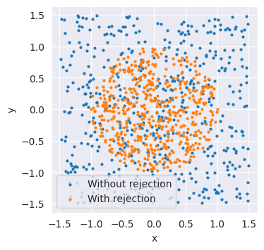
In some settings, we might want to exclude simulations after sampling, for example because we can already tell that they are not plausible. Using the rejection_sample() method, we can specify a predicate function to provide a mask for the samples we consider valid.

Let’s make up a simple example. In our simulator, we generate two uniformly distributed values, x and y. We only want to accept samples that lie inside a circle with radius one, which gives the condition \(\sqrt{x^2+y^2}\le1.\)

rng = np.random.default_rng(seed=2025)
def simulator_fn():
    return {"x": rng.uniform(-1.5, 1.5), "y": rng.uniform(-1.5, 1.5)}

def predicate(data):
    return np.sqrt(data["x"]**2+data["y"]**2) <= 1.0

simulator = bf.make_simulator(simulator_fn)

import matplotlib.pyplot as plt

samples = simulator.sample(500)
filtered_samples = simulator.rejection_sample(500, predicate=predicate, sample_size=100)
plt.figure(figsize=(3.8,3.8))
plt.scatter(samples["x"], samples["y"], s=4, label="Without rejection")
plt.scatter(filtered_samples["x"], filtered_samples["y"], s=4, label="With rejection")
plt.gca().set_aspect("equal")
plt.xlabel("x")
plt.ylabel("y")
plt.legend()

<matplotlib.legend.Legend at 0x74337df0f950>

../_images/3bb230ea9faf014809f8f27b4bf7c966a448b80f970de3967372edb391492163.png

print("Shapes without rejection:", {k: v.shape for k, v in samples.items()})
print("Shapes with rejection:", {k: v.shape for k, v in filtered_samples.items()})

Shapes without rejection: {'x': (500,), 'y': (500,)}
Shapes with rejection: {'x': (529,), 'y': (529,)}

The rejection_sample() method automatically ensures that we get at least the number of samples described in batch_shape. As the function produces sample_size samples before each filtering step, it will usually overshoot a bit, so that we get more samples than we requested. If this is not desired (e.g., for comparisons with a fixed number of training datasets), we have to discard the additional samples manually.

Caution: If you misspecify the predicate function, or it is too restrictive, sampling can take very long (or forever) until the desired number of samples is reached.

2.4. Summary#

BayesFlow offers convenient wrapper classes that allow combining functions into more complex generative models, as well as utilities for sampling. For more detailed information, take a look at the API documentation of the simulators module.