10. Posterior Estimation With Multimodal Data

Author: Valentin Pratz

Observed data can come in many forms, like single observations, multiple exchangeable observations or time series. A fusion network can combine all those forms into a joint learned summary space, by combining the outputs of different specialized summary networks. This requires some pre-processing steps, which we will demonstrate in this tutorial.

10.1. Toy Problem

We will construct a simple toy problem, in which we have to determine the mean \(\mu\) and the standard deviation \(\sigma\) of a two-dimensional Gaussian distribution. For this, we simulate data from two experiments:

• Experiment A: n_exchangeable exchangeable samples from the distribution.

• Experiment B: A time series of the cumulative sum of n_time_series draws from the distribution.

Both experiments will share the parameters \(\mu\) and \(\sigma\).

import bayesflow as bf
import keras
import numpy as np
import matplotlib.pyplot as plt

2025-07-13 08:18:33.287030: E external/local_xla/xla/stream_executor/cuda/cuda_fft.cc:477] Unable to register cuFFT factory: Attempting to register factory for plugin cuFFT when one has already been registered
WARNING: All log messages before absl::InitializeLog() is called are written to STDERR
E0000 00:00:1752394713.299740   37155 cuda_dnn.cc:8310] Unable to register cuDNN factory: Attempting to register factory for plugin cuDNN when one has already been registered
E0000 00:00:1752394713.303495   37155 cuda_blas.cc:1418] Unable to register cuBLAS factory: Attempting to register factory for plugin cuBLAS when one has already been registered
2025-07-13 08:18:33.317954: I tensorflow/core/platform/cpu_feature_guard.cc:210] This TensorFlow binary is optimized to use available CPU instructions in performance-critical operations.
To enable the following instructions: AVX2 FMA, in other operations, rebuild TensorFlow with the appropriate compiler flags.
2025-07-13 08:18:35.581201: E external/local_xla/xla/stream_executor/cuda/cuda_driver.cc:152] failed call to cuInit: INTERNAL: CUDA error: Failed call to cuInit: UNKNOWN ERROR (303)
INFO:bayesflow:Using backend 'tensorflow'

rng = np.random.default_rng(2025)


def prior():
    return {"mu": rng.normal(size=2), "sigma": rng.gamma(5, 0.1)}

def likelihood_a(mu, sigma, n_exchangeable=5):
    return {"observables_a": rng.normal(mu, sigma, size=(n_exchangeable, 2))}


def likelihood_b(mu, sigma, n_time_series=20, **kwargs):
    return {
        "observables_b": np.cumsum(
            rng.normal(mu, sigma, size=(n_time_series, 2)), axis=0
        ),
        "time_b": np.linspace(0.0, 1.0, n_time_series)[:, None],
    }

We construct a simulator from the prior and the likelihoods in the usual way.

simulator = bf.make_simulator([prior, likelihood_a, likelihood_b])

We can simulate and visualize a few example datasets:

n_examples = 3
data = simulator.sample(n_examples)

cmap = plt.cm.Set1
for i in range(n_examples):
    plt.scatter(
        data["observables_a"][i, :, 0],
        data["observables_a"][i, :, 1],
        marker="x",
        color=cmap(i),
        label=f"Dataset {i+1}",
    )
plt.title("Experiment A")
plt.xlabel("$x_1$")
plt.ylabel("$x_2$")
plt.legend();

fig, axs = plt.subplots(2, 1, sharex=True)
for i in range(n_examples):
    for j in range(2):
        axs[j].plot(
            data["time_b"][i, :, 0].T,
            data["observables_b"][i, :, j].T,
            marker="x",
            color=cmap(i),
            linestyle="dotted",
            label=f"Dataset {i+1}",
        )
        axs[j].set(ylabel=f"$z_{j+1}$")
axs[0].legend()
axs[1].set(xlabel="$t$")
fig.suptitle("Experiment B")
fig.tight_layout();

10.2. Summary Networks

We start by setting up the individual summary networks, which will be the backbones of the fusion network. For Experiment A, we use a SetTransformer, which is constructed for exchangeable observations. For Experiment B, we use a TimeSeriesTransformer, which is designed to handle time series data. For the latter, we set time_axis=-1, indicating that we will concatenate the time to the data at the end of the vector. We will do this below using the adapter.

summary_network_a = bf.networks.SetTransformer(summary_dim=6)
summary_network_b = bf.networks.TimeSeriesTransformer(summary_dim=6, time_axis=-1)

To combine the outputs of both networks, we define another neural network, the head. It will get the concatenated outputs of our summary networks as inputs.

summary_dim = 6
head = keras.Sequential(
    [bf.networks.MLP(widths=[128, 128]), keras.layers.Dense(summary_dim)]
)

Now, pass all the the networks to the FusionNetwork. We use a dictionary for the summary networks, so that we can specify which input belongs to which summary network. The keys can be chosen arbitrarily, here we use input_a and input_b.

summary_network = bf.networks.FusionNetwork(
    backbones={"input_a": summary_network_a, "input_b": summary_network_b},
    head=head,
)

10.3. Pre-processing with the Adapter

We now have to transform the simulator outputs to the structure required by BayesFlow:

• the parameter vector goes to inference_variables

• the inputs to the summary networks go to summary_variables

As we now have multiple simulator outputs with incompatible shapes, summary_variables has to be a dictionary with the keys we used above for the summary networks. So it should have the contents:

• input_a: pre-processed oberservations from Experiment A that are passed to the SetTransformer

• input_b: pre-processed oberservations from Experiment B that are passed to the TimeSeriesTransformer

Note that most transforms in the adapter cannot handle nested structures (i.e., dicts) for now, so we have to create the summary_variables dictionary after all pre-processing has been done.

The simulator outputs variables with the following shapes (3 is the batch dimension):

print(keras.tree.map_structure(keras.ops.shape, data))

{'mu': (3, 2), 'sigma': (3, 1), 'observables_a': (3, 5, 2), 'observables_b': (3, 20, 2), 'time_b': (3, 20, 1)}

adapter = (
    bf.adapters.Adapter.create_default(["mu", "sigma"])
    .rename("observables_a", "input_a")
    .concatenate(["observables_b", "time_b"], into="input_b")
    .group(
        ["input_a", "input_b"], into="summary_variables"
    )  # this transform should go last
)

The adapter produces the following output, just as we expect it:

print(keras.tree.map_structure(keras.ops.shape, adapter(data)))

{'inference_variables': (3, 3), 'summary_variables': {'input_a': (3, 5, 2), 'input_b': (3, 20, 3)}}

10.4. Training

We have a summary network and the appropriate adapter, which are the two parts in our pipeline that are different for multimodal problems. From now on, the pipeline works as in any other BayesFlow workflow.

workflow = bf.BasicWorkflow(
    simulator=simulator,
    adapter=adapter,
    summary_network=summary_network,
    standardize="all",
)

history = workflow.fit_online(epochs=50, validation_data=64)

INFO:bayesflow:Fitting on dataset instance of OnlineDataset.
INFO:bayesflow:Building on a test batch.

Epoch 1/50
100/100 ━━━━━━━━━━━━━━━━━━━━ 35s 51ms/step - loss: 2.7755 - val_loss: 1.0353
Epoch 2/50
100/100 ━━━━━━━━━━━━━━━━━━━━ 4s 38ms/step - loss: 1.3387 - val_loss: 1.1301
Epoch 3/50
100/100 ━━━━━━━━━━━━━━━━━━━━ 4s 42ms/step - loss: 1.2271 - val_loss: 0.6304
Epoch 4/50
100/100 ━━━━━━━━━━━━━━━━━━━━ 4s 43ms/step - loss: 0.9349 - val_loss: 0.4039
Epoch 5/50
100/100 ━━━━━━━━━━━━━━━━━━━━ 4s 36ms/step - loss: 0.7373 - val_loss: 0.2693
Epoch 6/50
100/100 ━━━━━━━━━━━━━━━━━━━━ 4s 37ms/step - loss: 0.6610 - val_loss: 0.2306
Epoch 7/50
100/100 ━━━━━━━━━━━━━━━━━━━━ 4s 37ms/step - loss: 0.6769 - val_loss: 0.1249
Epoch 8/50
100/100 ━━━━━━━━━━━━━━━━━━━━ 4s 40ms/step - loss: 0.5096 - val_loss: 0.1006
Epoch 9/50
100/100 ━━━━━━━━━━━━━━━━━━━━ 4s 38ms/step - loss: 0.2563 - val_loss: -0.1138
Epoch 10/50
100/100 ━━━━━━━━━━━━━━━━━━━━ 4s 35ms/step - loss: 0.0946 - val_loss: -0.2080
Epoch 11/50
100/100 ━━━━━━━━━━━━━━━━━━━━ 4s 37ms/step - loss: 0.0426 - val_loss: -0.4784
Epoch 12/50
100/100 ━━━━━━━━━━━━━━━━━━━━ 4s 38ms/step - loss: -0.0722 - val_loss: -0.3966
Epoch 13/50
100/100 ━━━━━━━━━━━━━━━━━━━━ 4s 42ms/step - loss: -0.1299 - val_loss: -0.6153
Epoch 14/50
100/100 ━━━━━━━━━━━━━━━━━━━━ 4s 41ms/step - loss: -0.1728 - val_loss: -0.3874
Epoch 15/50
100/100 ━━━━━━━━━━━━━━━━━━━━ 4s 41ms/step - loss: -0.3064 - val_loss: -0.8856
Epoch 16/50
100/100 ━━━━━━━━━━━━━━━━━━━━ 4s 41ms/step - loss: -0.2076 - val_loss: -0.3698
Epoch 17/50
100/100 ━━━━━━━━━━━━━━━━━━━━ 4s 41ms/step - loss: -0.3563 - val_loss: -0.3134
Epoch 18/50
100/100 ━━━━━━━━━━━━━━━━━━━━ 4s 42ms/step - loss: -0.2574 - val_loss: -0.8124
Epoch 19/50
100/100 ━━━━━━━━━━━━━━━━━━━━ 4s 37ms/step - loss: -0.3502 - val_loss: -0.8620
Epoch 20/50
100/100 ━━━━━━━━━━━━━━━━━━━━ 4s 36ms/step - loss: -0.3385 - val_loss: -0.8182
Epoch 21/50
100/100 ━━━━━━━━━━━━━━━━━━━━ 4s 38ms/step - loss: -0.3814 - val_loss: -0.7470
Epoch 22/50
100/100 ━━━━━━━━━━━━━━━━━━━━ 4s 43ms/step - loss: -0.4002 - val_loss: -0.7260
Epoch 23/50
100/100 ━━━━━━━━━━━━━━━━━━━━ 4s 38ms/step - loss: -0.5205 - val_loss: -0.7855
Epoch 24/50
100/100 ━━━━━━━━━━━━━━━━━━━━ 4s 36ms/step - loss: -0.5317 - val_loss: -0.9134
Epoch 25/50
100/100 ━━━━━━━━━━━━━━━━━━━━ 4s 37ms/step - loss: -0.5224 - val_loss: -1.0202
Epoch 26/50
100/100 ━━━━━━━━━━━━━━━━━━━━ 4s 38ms/step - loss: -0.5744 - val_loss: -0.9743
Epoch 27/50
100/100 ━━━━━━━━━━━━━━━━━━━━ 4s 37ms/step - loss: -0.5816 - val_loss: -1.0404
Epoch 28/50
100/100 ━━━━━━━━━━━━━━━━━━━━ 4s 38ms/step - loss: -0.6324 - val_loss: -1.0958
Epoch 29/50
100/100 ━━━━━━━━━━━━━━━━━━━━ 4s 36ms/step - loss: -0.6455 - val_loss: -1.1029
Epoch 30/50
100/100 ━━━━━━━━━━━━━━━━━━━━ 4s 39ms/step - loss: -0.6042 - val_loss: -0.9503
Epoch 31/50
100/100 ━━━━━━━━━━━━━━━━━━━━ 4s 35ms/step - loss: -0.7196 - val_loss: -1.1586
Epoch 32/50
100/100 ━━━━━━━━━━━━━━━━━━━━ 4s 35ms/step - loss: -0.7402 - val_loss: -0.6876
Epoch 33/50
100/100 ━━━━━━━━━━━━━━━━━━━━ 4s 36ms/step - loss: -0.7076 - val_loss: -1.0936
Epoch 34/50
100/100 ━━━━━━━━━━━━━━━━━━━━ 4s 35ms/step - loss: -0.7035 - val_loss: -0.9844
Epoch 35/50
100/100 ━━━━━━━━━━━━━━━━━━━━ 4s 36ms/step - loss: -0.7123 - val_loss: -1.2175
Epoch 36/50
100/100 ━━━━━━━━━━━━━━━━━━━━ 4s 36ms/step - loss: -0.7109 - val_loss: -1.1313
Epoch 37/50
100/100 ━━━━━━━━━━━━━━━━━━━━ 4s 37ms/step - loss: -0.8064 - val_loss: -1.2972
Epoch 38/50
100/100 ━━━━━━━━━━━━━━━━━━━━ 4s 35ms/step - loss: -0.7728 - val_loss: -1.2560
Epoch 39/50
100/100 ━━━━━━━━━━━━━━━━━━━━ 4s 36ms/step - loss: -0.7956 - val_loss: -1.0061
Epoch 40/50
100/100 ━━━━━━━━━━━━━━━━━━━━ 4s 37ms/step - loss: -0.8562 - val_loss: -1.1419
Epoch 41/50
100/100 ━━━━━━━━━━━━━━━━━━━━ 4s 36ms/step - loss: -0.8594 - val_loss: -1.1745
Epoch 42/50
100/100 ━━━━━━━━━━━━━━━━━━━━ 4s 37ms/step - loss: -0.8583 - val_loss: -1.2937
Epoch 43/50
100/100 ━━━━━━━━━━━━━━━━━━━━ 4s 35ms/step - loss: -0.8524 - val_loss: -1.2493
Epoch 44/50
100/100 ━━━━━━━━━━━━━━━━━━━━ 4s 35ms/step - loss: -0.9084 - val_loss: -1.2418
Epoch 45/50
100/100 ━━━━━━━━━━━━━━━━━━━━ 4s 36ms/step - loss: -0.8387 - val_loss: -1.2865
Epoch 46/50
100/100 ━━━━━━━━━━━━━━━━━━━━ 4s 35ms/step - loss: -0.8720 - val_loss: -1.2618
Epoch 47/50
100/100 ━━━━━━━━━━━━━━━━━━━━ 4s 35ms/step - loss: -0.8053 - val_loss: -1.3140
Epoch 48/50
100/100 ━━━━━━━━━━━━━━━━━━━━ 4s 37ms/step - loss: -0.9148 - val_loss: -1.2975
Epoch 49/50
100/100 ━━━━━━━━━━━━━━━━━━━━ 4s 38ms/step - loss: -0.8805 - val_loss: -1.3046
Epoch 50/50
100/100 ━━━━━━━━━━━━━━━━━━━━ 4s 35ms/step - loss: -0.9346 - val_loss: -1.3002

10.5. Evaluation

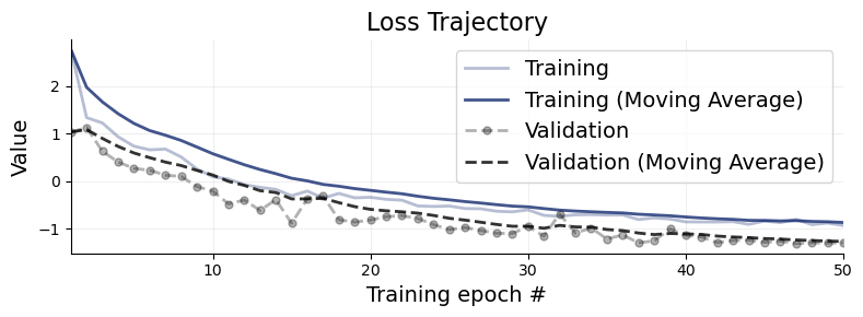
We plot the default diagnostic to assess whether training has been successful. Please refer to the introductory notebooks for details on the interpretation.

bf.diagnostics.plots.loss(history, figsize=(8, 3));

workflow.plot_custom_diagnostics(
    512,
    plot_fns={
        "recovery": bf.diagnostics.plots.recovery,
        "calibration_ecdf": bf.diagnostics.plots.calibration_ecdf,
    },
);